Display control
Compare six-color photo rendering on the OpenPaper 7 and see how to choose mixtures for an image.
Better photos with stock firmware
Tune how your project converts an RGB photo into the six colors of OpenPaper 7. The panel still receives ordinary black, white, red, yellow, blue and green pixels in a single full refresh. Start with the slider below, then use the measured palette and contrast curve to try it on your own image.
Default photo settings vs. tuned rendering
Drag across the cut orange, from the pale rind into the flesh. Check the deep shadow under the fruit as well as the brighter peel. Both sides are photographs of the same physical spot on a 7.3-inch panel running stock firmware.
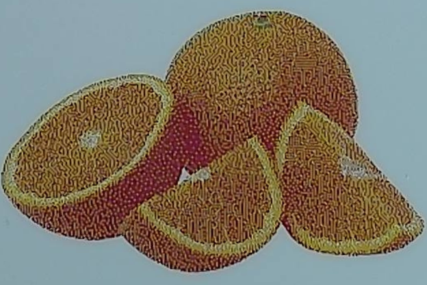
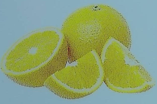
The default looks yellower and more saturated. The tuned rendering brings red back into the peel and separates light from shadow. Lightness contrast in the orange regions rose 32%. Average color error against the source fell from 20.73 to 5.37 ΔE₀₀, even though chroma fell 30%. Speckle is still visible up close. Paired measurements and capture conditions.
Use this rendering in a project
- Crop and resize the RGB image to its final pixel dimensions. For a full OpenPaper 7 image, use 800 × 480 in landscape.
- Model the six inks with their measured sRGB values. Convert to linear RGB and normalize each channel to the measured paper black and white.
- For the orange photo, apply an S-curve to lightness in the paper range (exponent 1.25) and multiply Lab chroma around the paper’s neutral axis by 1.30. Preserve black and white endpoints.
- Dither with serpentine Floyd–Steinberg using the measured colors to calculate error. Write each winning color’s native RGB code to the output PNG. Keep those pixels at their original size and bypass any second round of dithering. Curve, stronger setting and photo comparisons.
Download the OpenPaper 7 photo renderer (ZIP). Unzip it, then run the following in that directory on macOS or Linux. The defaults reproduce the tuned side of the slider.
python3 -m pip install numpy Pillow colour-science
cc -O3 -fPIC -shared diffuse.c -o diffuse.so -lm
python3 render.py cropped-photo.jpg device.pngMeasured colors in the ditherer
The center column of each group models black, white, red, yellow, blue and green by their ideal RGB values. The right column models the same six pixel codes using their measured appearance on this panel. Look at the astronaut’s face and the change in color between the coffee and the rim of the cup. Both versions were on screen together. The second capture swapped their physical positions.
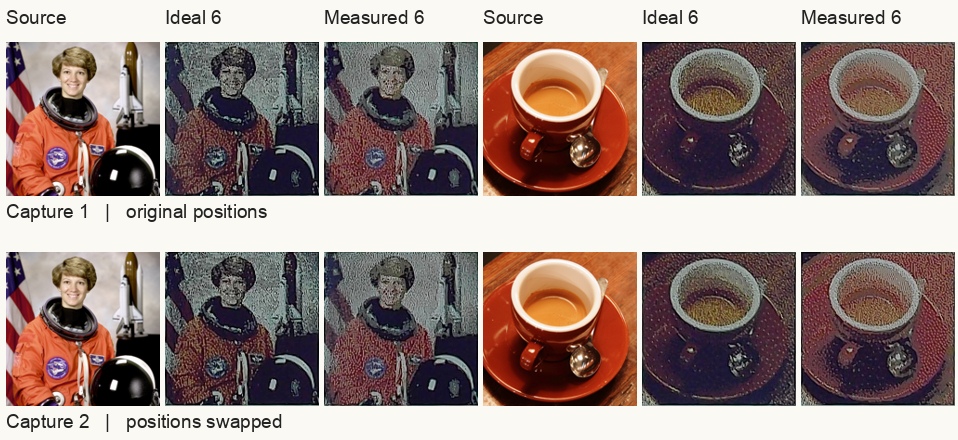
Grain fell 3.7% on average across eight uniform patches. The improvement depended on the color. Dark brown and teal became smoother in both captures, while brick red became grainier. Turning dithering off made the flat patches smoother still, but the face broke into blocks of green and white. Enlarged patch photographs and measurements.
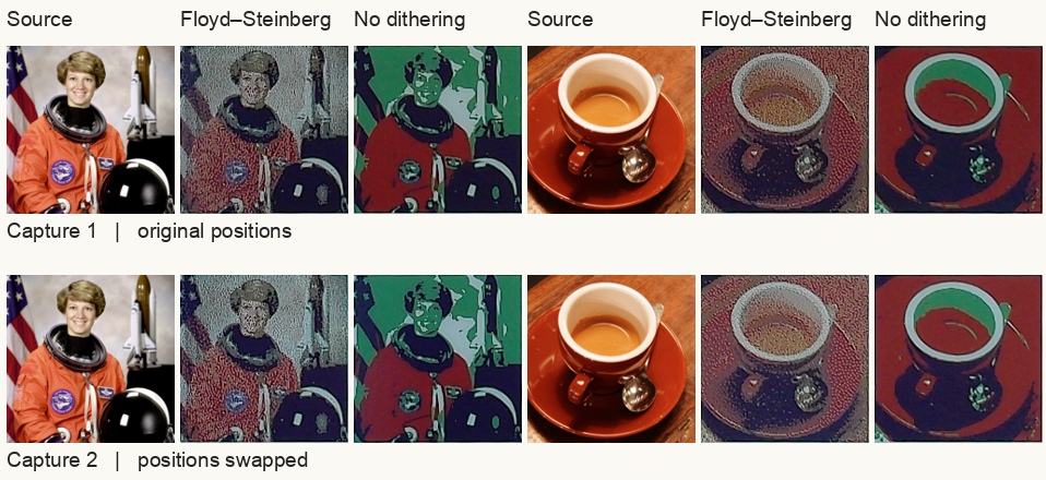
The stronger setting deepened the shadows further but increased average color error. See the strong-boost slider in Color Calibration.
Choosing colors for each image
A six-color frame can show an orange area by mixing pixels. In the tuned fruit, 71% of the pixels were red, 23% yellow and 5% white. Changing the mixture trades texture for accuracy. Restricting the fruit to red and yellow made flat patches smoother, while allowing neutral pixels helped match the source color. For photos with several hues, the measured six-color palette gives the ditherer access to all six inks. Mixture photographs and results.